


Article by Jason Mueller
Part 1: Quantum simulations
Quantum computing is a computational paradigm which encodes information into quantum systems called qubits. These qubits are manipulated using superposition and entanglement to achieve a computational advantage over classical computers. In particular, photonic qubits are one of the most promising quantum-computer technologies [1], with billions invested across the world. As the field continues to evolve quickly, the need to efficiently simulate the calculations performed by quantum circuits becomes evermore pressing.
Perceval, the software layer of Quandela’s full-stack quantum computer, allows you to simulate quantum circuits, their outputs, and to write and run quantum algorithms. The simulator includes several backends, each tailored to the different kinds of algorithms you may be interested in running [2]. Here, we’ll be learning about Perceval’s Strong Linear Optical Simulation (SLOS) backend, which allows us to time-efficiently simulate the output distribution of linear optical quantum circuits, with applications ranging from quantum machine learning to graph optimization [3].
Part 2: Why SLOS?
First, what is the difference between a strong and a weak simulation? Consider the simple example of rolling a die, where we want to know the probability of its landing on each face. There are two options: roll the die many times and write down the number of times each face turns up, or write down the precise probability that each face appears based on physical knowledge we have about the die (e.g. number of faces, shape of die). The first case of rolling the die many times is called a weak simulation, because we’re learning about a probability distribution by sampling from it, one trial at a time. The second case of writing down the precise probabilities is called strong simulation, because we have fully characterized the behavior of the die without sampling.
Now imagine that instead of a die, you had a photonic circuit like the one shown in Fig. 1, which includes indistinguishable photons through modes.

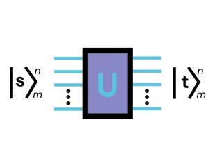
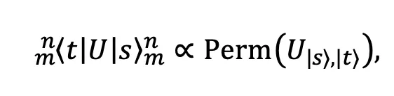
The output distribution is proportional to the permanent:

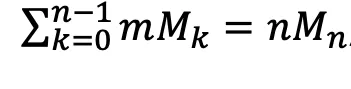
Using SLOS, we can improve on the complexity of brute-force algorithms, which calculate each output state individually, by an exponential factor of 2ⁿ. SLOS computes several inputs and outputs directly, with the time-scaling 𝒪(nMₙ), where Mₙ = C(n+m-1, m-1) is the binomial coefficient.
Part 3: SLOS_full and SLOS_gen
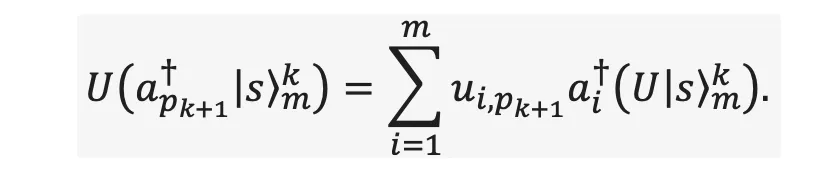
Perceval includes two versions of SLOS: SLOS_full, which iteratively calculates the full output distribution, and SLOS_gen, which recursively calculates the output distribution given some constraints. The mathematical key to both of these algorithms is understanding how we can efficiently decompose

where pₙ is the position of each photon that is created. For k < n-1 photons, we can add one more photon to our state as
Finally, we concatenate this product:
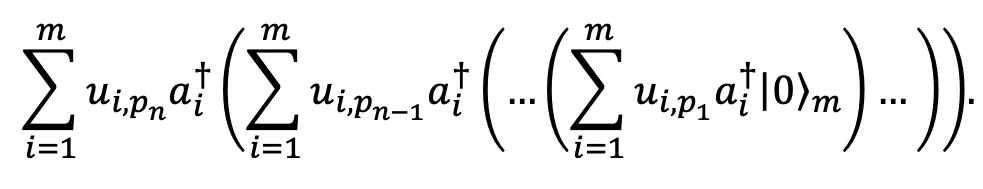
More simply, SLOS_full calculates and stores the coefficients of a state with photons, then extrapolates to the next state of photons — the specific algorithm is given in [3]. The complexity of SLOS_full is that given a state with photons, you have ways to put in the photon:
which is linear in the number of states!
But suppose you’re interested in only a few of the output modes, common for algorithms which rely on heralding or post-selection. SLOS_gen is the solution. This version of SLOS introduces a mask to filter the states at each step of the computation: we compute the coefficients of a full k-photon state, then we apply the mask so that we obtain only the k-1 -photon states that we’re interested in, then we compute the now-reduced k-photon coefficients and continue. While this algorithm does introduce a memory overhead because it is recursive, the average complexity still scales as 𝒪(n2ⁿ).
Part 4: Complexity vs. Memory
SLOS exponentially outperforms other state-of-the-art approaches, with the tradeoff being that it requires a large memory. The memory requirement of SLOS_full is 𝒪(Mₙ); for n = m = 12, M₁₂ = 1.35 × 10⁶.
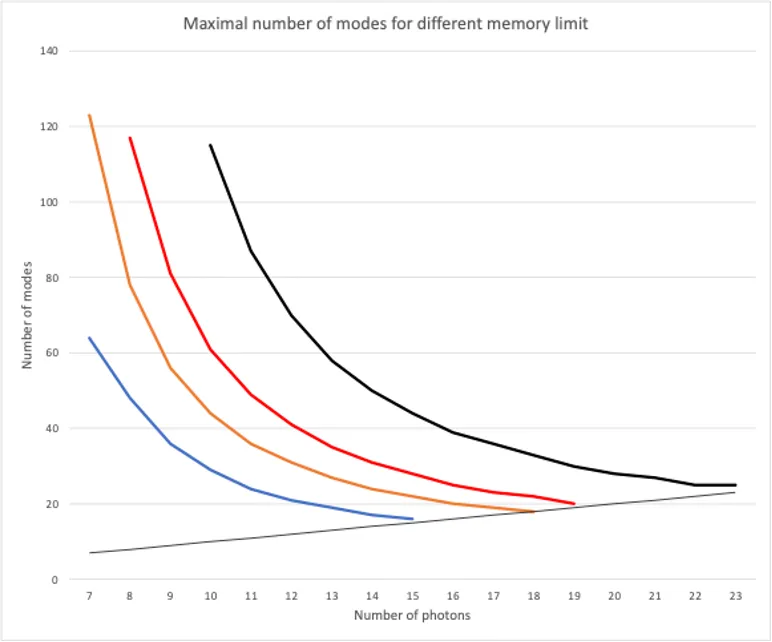
The memory complexity of SLOS_gen is difficult to calculate due to state redundancy, but for a single input and output, there are C(n, n/2) coefficients to be stored. To visualize these memory constraints for typical computers, we show the maximum state size allowed for a given memory in Fig. 2 — the maximum number of photons and modes that a laptop can practically calculate is ~12.
Part 5: SLOS in action!
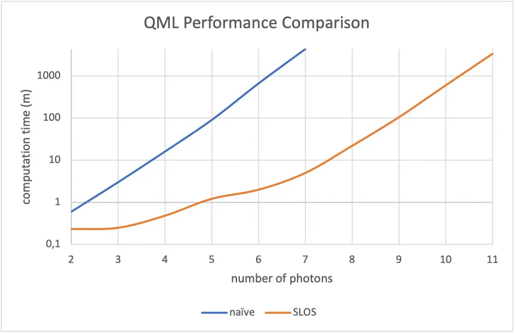
Let’s see how SLOS performs on a typical quantum machine learning application, where we want to train a quantum circuit to approximate the solution of a differential equation [7]. This requires repeatedly calculating the full output distribution, optimizing the circuit configuration each time. The algorithm converges in 200 to 400 iterations, each with thousands of full-distribution calculations! When we compare the performance of the traditional approach used in the original research versus SLOS, we see that the number of calculable photons is improved from 6 to 10 (see Fig. 3). Put another way, if you are interested in using 6 photons for the simulation, the SLOS optimization takes only 2 minutes, a factor-330 time improvement over the original method.
Part 6: Where and how to use SLOS
Although SLOS is memory-intensive, it is a complexity-efficient backend, unique to Perceval, for simulating output distributions of linear optical circuits. The 2ⁿ time advantage offered by SLOS is useful for researchers to simulate their theories and verify their experiments, and it is useful for industry to quickly design and validate algorithms.
You can access SLOS through the open-source code on GitHub [8]. Quandela’s tutorial center also includes several applications using SLOS [9–12], which you can run both locally and on Quandela’s quantum cloud service [13].
References:
[2] Computing Backends — perceval 0.3.0a2 documentation (quandela.net)
[3] [2206.10549] Strong Simulation of Linear Optical Processes (arxiv.org)
[7] [2107.05224] Fock State-enhanced Expressivity of Quantum Machine Learning Models (arxiv.org)
[8] GitHub — Quandela/Perceval: An open source framework for programming photonic quantum computers
[9] Differential equation resolution — perceval 0.3.0a2 documentation (quandela.net)
[10] Boson Sampling with MPS — perceval 0.3.0a2 documentation (quandela.net)
[11] Using non-unitary components in Perceval — perceval 0.3.0a2 documentation (quandela.net)
[12] Remote computing with Perceval — perceval 0.3.0a2 documentation (quandela.net)
[13] Welcome to Quandela Cloud
If you are interested to find out more about our technology, our solutions or job opportunities visit quandela.com