Article by Sebastien Boissier

Benchmarking Single-Photon Sources

In the span of twenty years, we have witnessed an extraordinary emergence of quantum information technologies — the beginning of what some have called the second quantum revolution. Technology that was once the exclusive playground of scientists is now becoming accessible to a broad range of end-users.

This is good news because progress can be best sustained when the enabling technology is readily available to the broader research and development community. In the quantum realm, the manipulation of isolated quantum objects (atoms, electrons, photons, etc.) and control over their unique properties (entanglement, quantum superposition, non-locality, etc.) is becoming increasingly accessible owing to the development of new products.

To support the growing quantum ecosystem, Quandela is developing and commercialising sources of optical qubits based on single photons. These quantum light sources are crucial building-blocks for optical quantum technologies. To give some examples, they can enable truly-random number generation, enhanced imaging and sensing methods, secure quantum communication and scalable quantum computing.

Quandela offers the brightest single-photon sources available on the market to help researchers and businesses unlock useful quantum applications.

In this post, we will first approach single-photon sources from a conceptual level so that we can identify and understand their key properties. Then we will go on to explain some of the various performance metrics often quoted in the literature. This is important for anyone wishing to compare different kinds of photon source.

Desiderata

First let’s discuss some key properties to keep in mind when assessing single-photon sources.

Property #1: Single-Photon Purity

As the name suggests, we expect a single-photon device to produce one, and only one, particle of light at a time. This is very important because the presence of additional photons leads to errors in quantum protocols that are designed to work with precise numbers of photons.

Purity is a much harder requirement to fulfill than one might imagine. For example, we cannot build a good single-photon source by simply dimming a laser or a candle. Even if a laser beam is attenuated to the point where there is on average much less than one photon at any given time interval, the statistics are such that there is still an unacceptable probability of having more than one. So a true single-photon source must actively suppress the probability of multi-photon emission, while maximizing the probability of having just one.

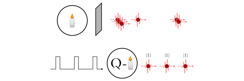
Property #2: Photons-on-Demand

Another important requirement is that the source must be triggered. Advanced quantum-photonic protocols rely on interference effects between two photons, which typically occur on a beam-splitter (a semi-reflective mirror). To interfere, photons must arrive at the beam-splitter at the same time and that requires synchronisation. We must therefore control the emission time of the photons with a trigger.

Typically, single-photon sources may be triggered by a pulsed laser that stimulates the emission of single-photons at precise time intervals.

Property #3: Brightness

More than requiring photons on-demand, we wish for a high probability that the source emits once we do pull the trigger. This property is what is known as brightness.

It is obvious that ending up with no photons is not very useful. But obtaining a high brightness is perhaps the most difficult challenge to address, mostly because photons are very easy to lose. And for certain sources, brightness is a trade-off against a higher probability of multi-photon emissions.

Source brightness is crucial for the scalability of optical quantum technologies, since differences in the brightness have an exponential effect on performance as we increase the complexity of our protocols by adding more sources to them. Therefore even small gains in brightness can have drastic improvements for experiments with a large number of sources.

Property #4: Indistinguishability

On the topic of interference, it turns out that for two photons interfere they should ideally be completely identical to one another in all degrees of freedom. These includes polarisation, as well as spectral and spatial envelopes. This indistinguishability condition puts harsh constraints on the sources. For two photons to be exactly identical, the emission process must itself be precisely reproducible.

Metrics

Now let’s see how we can put some numbers to the properties discussed above.

Purity

An important tool for assessing single photon purity is the second-order correlation function g⑵. Correlation functions are used to characterise the statistical and coherence properties of light. While a full treatment requires more space than a blog post, a first order approximation of g⑵ for high-performing triggered source is g⑵ ≈ 2 P(2) / P(1)² where P(n) is the probability of having n photons per triggering event. So a g⑵ measurement gives us a good idea of the probability that a source malfunctions by emitting two photons.

[Note that strictly speaking P(1) differs from the brightness B because most detectors only register the presence of photons but not the number of them. To complicate matters, however, some papers ignore this distinction and define B as P(1).]

But why use this metric instead of directly quoting the probabilities P(1) and P(2), etc.? Well, it turns out that this first order approximation of g⑵ can be measured in the lab with a rather simple apparatus, shown below:

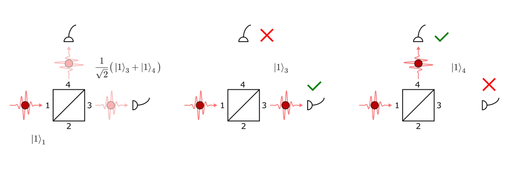
The experiment consists of sending a single photon to a beam-splitter. The action of the beam-splitter is to evenly split the photon’s wavefunction into a superposition of two distinct paths. If we observe the photon at one detector, the wavefunction collapses into the corresponding branch of the superposition and no photon is detected on the other path. So for single photons we should never observe coincidence events at the two detectors.

But let’s suppose the source has less than perfect purity and see what happens if two photons arrive at the beam-splitter:

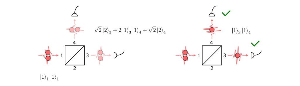
In this case, the wavefunction contains a term in which one photon exits in each path. Half of the time the wavefunction collapses to this branch and we can expect both detectors to fire.

Suppose we are working with a good source which is triggered. We observe that the probability per pulse of detecting a photon at one detector is C₁, and that the probability per pulse of having both detectors firing simultaneously is C₂ . Then to a good first approximation g⑵ ≈ C₂/(C₁)². For perfectly pure single-photon emissions there would be no coincidence events, C₂ = 0, and we would find g⑵ = 0 as expected. In practice the aim is for this figure to be as low as possible.

Above we show an example of a g⑵ measurement done in our labs. Here, we trigger a single-photon source with a constant repetition rate and we send the outputs of the two single-photon detectors to a coincidence time-correlator. The correlator’s job is to measure the time delay between a photon arriving on one of the detectors and the next photon arriving on the other detector. We collect many such time differences and plot them in a histogram.

In this histogram we can clearly see the repetition rate of our source, as photons emitted in different pulses can trigger both detectors albeit with a time delay. However, we see very little coincidences around zero time-delay which is the quantum signature of our single-photon source.

Brightness

Typical sources are triggered at a constant repetition rate R (number of triggering events per unit of time). With a source of brightness B (a probability lying between 0 and 1) we would end up with a single-photon count rate G = B * R .

Often, the count rate is measured at the output of a single-mode fibre which acts as a “wire” for photonic technology. So knowing the repetition and count rates would allow us to infer the brightness.

However, detecting photons is also an imperfect process. Although single-photon detectors are a relatively mature technology, there still is a small probability that the detector does not register the presence of a photon even when one is present. For state-of-the-art detectors, the detection efficiency μ can be very close to 1 (detectors for which μ > 0.95 already exist).

Therefore our detected count rate is D = μ * B * R . So if we have the detected count rate, detector efficiency and repetition rate, it is then easy to deduce the brightness of a source.

But what if we wanted two photons in our experiment? Then we have a two-photon coincidence rate D₂ = (μ * B)² * R , as we have to multiply the probabilities that two sources successfully emit a photon and that two detectors register the emission.

More generally, we have an n-photon coincidence rate Dₙ = (μ * B)ⁿ * R . The term (μ * B)ⁿ decays exponentially with increasing number of sources. It is therefore crucial to have B as close to 1 as possible, and incremental improvements of B lead to huge gains in multi-photon coincidence rates.

Indistinguishability

Finally, we need a number to quantify the degree of similarity between photons. As we mentioned before, this is critical for building complex protocols based on photon interference. Photon indistinguishability is typically measured by a Hong–Ou–Mandel interference experiment.

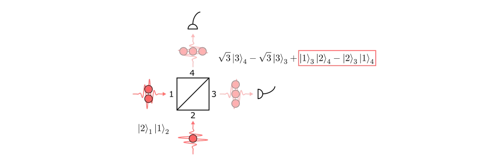
In this setup, two photons arrive at the same time via different ports of the beam-splitter. To see what happens we must first understand the full action of the beam-splitter.

Notice that the beam-splitter acts slightly differently on a photon entering by port 1 than it does on a photon entering by port 2. A minus sign appears for the reflected term of the wavefunction for a photon that entered through port 2. This so-called Stokes relation is a consequence of the time-reversal symmetry of the Maxwell equations (for lossless materials).

If we expand the output state in the case that a photon enters via each port, we find:

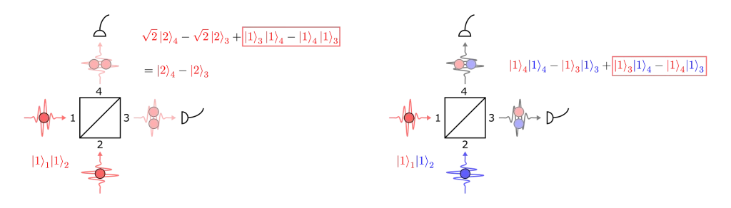
Here we have separated the cases where the input photons are identical or different (after all this is what we are trying to measure).

If we have indistinguishable photons, then apart from having opposite signs there is no way to distinguish the final two terms… and their probability amplitudes cancel out! We are therefore left with an entangled state, which gives zero probability of measuring coincidences between the two detectors.

If on the other hand the two photons are distinguishable, then there is not a total cancellation between final terms, and we do observe coincidences.

So the coincidence rate in this experiment indicates how distinguishable the photons are. Usually it is simpler to speak in terms of the Hong–Ou–Mandel (HOM) visibility Vₕₒₘ, which essentially corresponds to the non-coincidence rate, and which indicates how indistinguishable the photons are.

A low number of coincidences means a high Vₕₒₘ, and Vₕₒₘ is equal to 1 only if we see no coincidences at all. For complex quantum protocols to work without being overwhelmed by errors, we should aim to have Vₕₒₘ as close as possible to 1.

It is also important to mention that the HOM visibility can be corrupted by the presence of more than one photon in the input ports. For example, consider the following scenario:

With an extra photon in port 1, we would get a state where coincidences are again possible. So even if a source emitted perfectly identical photons but was not perfectly pure — i.e. had some probability of emitting two at a time (g⑵>0) — then we would not measure a perfect HOM visibility.

When trying to understand why a source doesn’t have Vₕₒₘ=1 it is usually a good idea to separate out contributions due to impurity from contributions due to distinguishability. In the literature, therefore, we often find values for the corrected HOM visibility. The correction is so that we only take account of the contributions due to distinguishability.

Here is the result of an HOM interference measurement with one of our triggered sources. Here we precisely delay every other photon (approximately) such that two photons of the same source arrive at the beam-splitter at the same time. We then use the same coincidence correlator as for the g⑵ measurement to build up the histogram.

Again we see the repetition rate of the source as photons which do not arrive at the same time on the beam-splitter do not interfere. At zero time-delay, we do not see many coincidences which is the sign that our photons have bunched together at the output of the beam-splitter.

Summing Up

In conclusion, we have looked at the three key features of a single-photon sources: single-photon purity, indistinguishability, and brightness, and we have introduced respective metrics for assessing these: the g⑵ correlation function, the brightness as inferred from various count rates, and the HOM visibility Vₕₒₘ.

So where do we currently stand in terms of these performances? As we will see in the next posts, there are two main technologies able to produce high quality single-photons: quantum-dots in micro-cavities and spontaneous optical frequency down-conversion. Here is a rough map of the progress being made towards the ideal single-photon source:

To Be Continued

In the next post in this series we will introduce one of the technologies that has been developed to create single photons: heralded photon-pair sources with active multiplexing.