Article by Sebastien Boissier

Heralded Sources and Multiplexing

Welcome to part two of our series on single-photon sources. Here, we will discuss one possible route for single-photon generation: spontaneous photon-pair sources.

Non-linear optics

To understand spontaneous photon-pair sources we have to delve into how dielectric material react to light. Classically, light is nothing but the synchronised oscillations of electric and magnetic fields. And dielectrics are electrical insulators which can be polarised by an electric field. Let’s try to unpack these concepts.

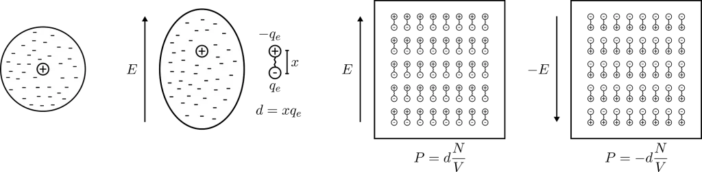
When an electric field E is applied to a dielectric material, the electrons within the material’s atoms are pulled away from their respective nuclei but without being able to escape (because dielectric materials are insulators). This creates many dipoles (pairs of positive and negative charges separated by a small distance) and we say that the material is polarised.

The macroscopic strength of these dipoles is described by the polarisation density P which is given by P = x * qₑ * N/V where x is the separation between to charges, qₑ is the negative charge (assuming the charges are opposite but equal in magnitude) and N/V is the density of dipoles (number of dipoles per unit volume).

Let’s now assume we have a perfectly monochromatic laser beam oscillating with an angular frequency ω and traveling through the dielectric. In complex notation we can write this as

where c.c. is the complex conjugate of the term in front. In response to the oscillating electric field, the electrons and nuclei also start to oscillate, and we get a bunch of oscillating dipoles which in turn lead to a macroscopic polarisation density P(t) that oscillates. It is typically assumed that P(t) depends linearly on the external electric field, so that

where the constant of proportionality ꭓ⑴ is known as the linear susceptibility of the material and 𝜖₀ is the permittivity of free space. The important take-away here is that the dipoles oscillate at the same frequency than the laser.

What’s more, oscillating dipoles are nothing but accelerating charges which themselves emit electromagnetic radiation. It turns out that the dipoles act as a source of light Eₚₒₗ(t) which oscillates at the same frequency as P(t). This new field then gets added to the external driving field.

We therefore have the following string of cause-and-effect Eₗₐₛₑᵣ(t) → P(t) → Eₚₒₗ(t) which produces the output field Eₗₐₛₑᵣ(t)+Eₚₒₗ(t) where the two components oscillate at the same frequency.

In some dielectrics and at high driving power (large Eₗₐₛₑᵣ), the linear relationship between Eₗₐₛₑᵣ(t) and P(t) breaks down. We now enter the nonlinear regime where the relationship is better approximated by adding extra terms in the power series expansion like so

Note that ꭓ⑵ and ꭓ⑶ are typically a LOT smaller than ꭓ⑴ in magnitude. Focusing on the ꭓ⑵ non-linearity and expanding the squared term we get

In this regime, the dipoles not only oscillate at the frequency of the driving laser but also pick up another frequency component at 2ω. The result is that light is emitted at a different frequency than what had been sent in the material. In this case, we get second-harmonic generation.

So what is happening at the level of the photons? Recall that the energy of a photon is given by ħω where ħ is the reduced Planck’s constant. Here we’re assuming that the material is transparent (that it does not absorb energy), so in order to conserve energy two laser photons at frequency ω must be absorbed to generate a photon at frequency 2ω.

Another interesting thing happens when we drive the dielectric material with two laser beams at different frequencies:

Again, focusing on the ꭓ⑵ non-linearity and expanding the squared term, we get terms that oscillate at frequencies ω₁+ω₂ and ω₂-ω₁ (assuming ω₂>ω₁). This is called sum- and difference-frequency generation. Sum-frequency generation is easily understood as one photon from each driving field being absorbed to produce a photon at ω₁+ω₂.

Difference-frequency generation is a little more interesting. During this process, one photon at the pump frequency ω₂ is absorbed and two photons are emitted, one at the driving frequency ω₁ (the signal photon) and the other at ω₂-ω₁ (the idler photon).

Spontaneous parametric down‑conversion

If we attenuated the signal field (ω₁) down to zero, we would not expect any difference-frequency generation to occur. However, the electromagnetic vacuum is not completely empty and at the quantum level there are vacuum fluctuations. These fluctuations correspond to the momentary appearance of particles (in our case photons) out of empty space, as allowed by the uncertainty principle.

It turns out that vacuum fluctuations cause difference-frequency generation in ꭓ⑵ dielectrics without the presence of a signal field. This process is called spontaneous parametric down‑conversion and leads to one photon in the pump field being absorbed and a photon pair being emitted. Parametric just means that no energy is absorbed by the material, and the process is spontaneous because we cannot control when and where in the crystal the down‑conversion will occur (like all the other nonlinear processes).

Because we don’t have a second reference frequency any more, it’s fair to ask at what frequencies the photons will emerge. In addition to respecting conservation of energy, the photons involved in the down‑conversion process must also obey conservation of momentum. The momentum of a photon is given by ħk where |k|= n(ω) * ω / c is called the wavevector and it depends on the material’s refractive index n at the frequency of the photon (c is the speed of light).

Momentum conservation dictates that k(ωₚ)=k(ωₛ)+k(ωᵢ) (where the subscripts p, s and i correspond to the pump, signal and idler photons respectively), and because of material dispersion and birefringence this condition is only satisfied for certain frequencies, directions and polarisation of the photons (and they need not be the same for the signal and idler).

Conservation of momentum is also referred to more broadly as phase-matching. In general, the properties of the signal and idler photons satisfying energy and momentum conservation are usually not the ones we want. To solve this, we must engineer the nonlinear material and the setup to achieve phase-matching for the correct output frequencies. This can be done by birefringent phase-matching, by engineering the dispersion profiles of optical modes and with quasi-phase-matching.

Materials with large ꭓ⑵ coefficients required for spontaneous parametric down‑conversion are usually rather exotic. Common choices are lithium niobate (LiNbO3), potassium titanyl phosphate (KTiOPO4) or aluminum nitride (AlN).

It is also possible to use higher non-linear coefficients to achieve a similar effect. The other popular choice is spontaneous four-wave-mixing in ꭓ⑶ materials. More common materials, like silicon, have large ꭓ⑶ coefficient which makes this process an appealing alternative.

Spontaneous photon-pair sources as emitters of single photons

The discussion so far has been quite removed from the topic of single-photon sources. In this section we finally answer why spontaneous photon-pair sources can be useful in that regard.

Two-mode squeezed-vacuum

First, let’s recall (see part 1 of the series) that sources of single photons have to be triggered. By exciting a ꭓ⑵ dielectric with a continuous laser, spontaneous parametric down‑conversion does not allow us to control the emission time of a photon pair.

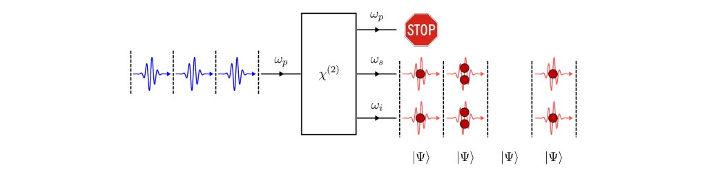
A better alternative is to restrict the emission to time slots defined by laser pulses. The nonlinear process can only take place when the laser is “on” and that acts as our trigger. However, we cannot completely control whether a photon-pair is emitted within one laser pulse or if we get multiple pairs.

In fact, if we can separate the down-converted photon from the pump light, the photon-number state that we get in each pulse is (ignoring the spectral, momentum and polarization degrees of freedom)

This state is called the two-mode squeezed-vacuum state and the parameter λ (called the squeezing parameter) is a number between 0 and 1 which quantifies the strength of the interaction. λ depends on the ꭓ⑵ nonlinearity, the interaction length and the laser power. Note that the two-mode squeezed-vacuum state is an entangled state in photon number.

Assuming that λ is small, we can approximate the emitted state as

From this, we can directly calculate the probabilities of getting one or two pairs in the time slot defined by a laser pulse. We have to square the amplitudes to get probabilities, so P(1 pair)≈λ² and P(2 pairs)≈λ⁴.

If we separated the signal and idler photons, could we use either of them as a single-photon state? Well, we are not off to a great start because we have some probability of having more than one photon-pair per laser pulse. In fact, if we completely ignored one of the outputs of the down‑conversion process (say the signal photons), the idler photons would have

Remember that a single-photon source needs a g⑵ as close to 0 as possible to avoid errors in our quantum protocols. A g⑵ equal to 2 is bad. In fact, it’s worse than if we had just used strongly attenuated laser pulses directly, which have g⑵=1.

Heralding

This can be redeemed if we use the photon-number entanglement in the two-mode squeezed-vacuum state. The trick is to monitor one of the outputs (say the signal) and record which output pulses have one or more photons. If we detect signal photons in a particular time slot, we now know that there is at least one photon in the idler path.

So, conditioned on the detection of a signal photon (or photons), the state of the idler collapses to the mixed state

where we have used the density matrix formalism. The vacuum component is projected out.

This time, the g⑵ of the idler photon is

And there we have it. By heralding the presence of idler photons with the signal photons, we get a state that approximates a single-photon state asymptomatically better as λ² tends to zero.

However, recall that the probability of getting a single-pair per pulse is also related to λ² (in fact it is equal to λ²) . This is an important compromise we have to make with spontaneous photon-pair sources: we have to keep the brightness of the source low in order for the single-photon purity to be high. It’s a trade-off between scalability and algorithmic errors. For example, if we wanted P(1) to be 10%, then g⑵=0.2 and that’s quite high for a single-photon source.

Note that this can be improved with the use of photon-number resolving detectors, which not only measure if there are photons but also how many. By heralding only the single-photon events in the signal paths (and rejected the vacuum and multi-photon components), we can decrease the g⑵. Even so, the statistics of the two-mode squeezed-vacuum state as such that the theoretical limit for brightness is 25%.

Spectral purity

Heralding is a great way to turn spontaneous photon pair sources into single-photon sources. However, it also creates additional constraints on the nonlinear process. Let’s focus on the frequencies of the emitted photon pair. In general, the emitted state is given by

where f(ωₛ, ωᵢ) is called the joint-spectral-amplitude. If f(ωₛ, ωᵢ) is not factorable — i.e. f(ωₛ, ωᵢ)≠ f(ωₛ)* f(ωᵢ) — the photons are entangled in frequency and measuring the signal photon collapses the idler to a mixed state, generally written

Mixed states in frequency are not a problem for photon purity. A single-photon, regardless of its frequency state, will only be measured at one output of a beam-splitter, and therefore has g⑵=0 (see part 1). However, it is bad for its Hong–Ou–Mandel visibility. A mixed state essentially means we have classical probabilities pₙ of getting different quantum states every time. And distinguishable states will not produce perfect interference on a beam-splitter (again, see part 1). In general, the detection of the signal photon must teach us nothing about the state of the idler photon except for its presence.

To have a spectrally-pure idler state, we have to work harder to engineer a factorable joint-spectral-amplitude. This can be done with group-velocity matching and apodization of the joint spectral amplitude by engineering the profile of the nonlinear medium. Another good method is to further engineer waveguide modes and using long interaction lengths.

Failing to produce a factorable spectrum, we can always filter the output photons to reject all possible frequency states but one. While this approach improves spectral purity and therefore indistinguishability, it comes at the cost of reducing the brightness of the source and that compromises its scalability even more.

Multiplexing

The balance between brightness and single-photon purity seems to be a major hurdle for spontaneous photon-pair sources. Is this the end of the story? No, because we can improve the efficiency of these sources by multiplexing.

At its core, multiplexing is a simple idea. Instead of using just one time-bin of one photon-pair source, we combine multiple sources (spatial multiplexing) or incorporate several time-bins of the same source (temporal multiplexing) to produce a better single-photon source. We consume more resources for better performance. Let’s quickly talk about both options.

Spatial Multiplexing

With spatial multiplexing, we first have to build a number of identical photon-pair sources. It is important that all the heralded single-photon outputs are the same or the indistinguishability of the multiplexed source will suffer.

Once that’s done, the output of the sources are connected to a reconfigurable routing-circuit (a multiplexer). All the sources are then pumped simultaneously with laser pulses and we monitor the emission of signal photons. We then pick one of the sources which has fired and route its now-heralded idler photon to the output of the circuit.

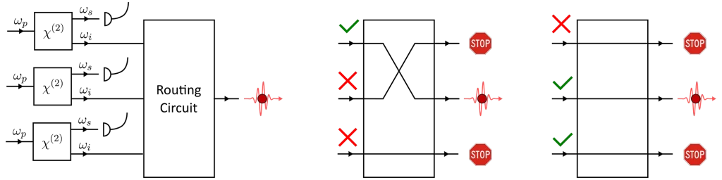
Because we have multiple sources working together, the probability that at least one fires can be a lot greater that the brightness of the individual sources. In fact, assuming a perfect routing circuit the brightness is improved by

where B₁ is the brightness of the sources and N is the number of sources hooked-up to the routing circuit.

Things now look at lot better, but we do have to consume a lot of resources. Say we want a source with g⑵=0.05 (that’s not bad for the state-of-art), then B₁ ≅ P(1) = 2.5% and we need at least 15 sources for a final brightness of 30% (28 for 50% and 91 for 90%).

Temporal Multiplexing

The other variant of this technique is temporal multiplexing. Here, we use contiguous time-bins of the same source (recall that we pump the sources at regular time intervals). We simply wait for the source to fire in one of the time-bins and delay the heralded idler-photon accordingly so that it leaves the circuit in a known time-bin.

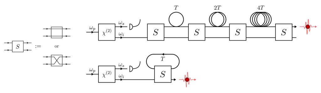
The overall effect is the same as for spatial multiplexing but N is now the number of time-bins that we use. One key advantage of temporal multiplexing is that sequentially emitted photons of the same source are usually more similar than those emitted by different sources, which helps with indistinguishability. The price we pay however is a decrease in the repetition rate of our source which goes from R to R / N.

Repetition rates are important in quantum photonics because experiments are usually probabilistic. We typically known when a particular run has succeeded but we could wait a while for that to happen. The ability to perform the experiment as often as possible is therefore desirable. This is what we are sacrificing with time-multiplexing.

We could also have anything in between full-temporal and full-spatial multiplexing depending on the scarcity of our two resources (experiment time vs number of sources).

Outlook

As can be seen in figures above, multiplexing can be wasteful. As we add more sources (or time-bins) to boost the brightness, we also increase the probability that two or more sources fire in the same multiplexing circuit. Unfortunately, we have to discard these photons because trying to route them to a second exit (or time-bin) will just add complexity and result in an additional source which has a poor brightness.

One interesting idea to improve this is that of relative multiplexing. In this scheme, we do not force the sources to always emit in the same exits or time-bins. Instead, we correct the relative distance (in space or in time) between photons that have been heralded. By using more of the emitted photons, we can reduce hardware complexity while improving coincidence counts.

It must be said however that multiplexing relies on the ability to integrate high-performing photonic components at scale. To implement a routing circuit, we must have access to optical switches, delay lines, single-photon detectors, fast electronics, etc… At present, photonic components can be lossy and/or slow to operate. This limits the performance of multiplexing, and we have to use even more hardware to reach the required improvement in brightness.

Summary

In summary, we have looked at how spontaneous photon-pair sources can generate single photons. We have seen how these sources are probabilistic, in the sense that we cannot completely eliminate the probability of multi-photon emission. In addition, it is only when the presence of one photon is heralded by the detection of the other that these sources become useful for single-photon generation.

We also described how the brightness of these heralded sources has to be kept low in order for the purity of the emission to be high. This can be remedied by multiplexing, but at the cost of multiplying the number of components, and therefore limiting the scalability in the long run.

Heralded photon-pair sources are very much still an active and ongoing topic of research, both theoretically and experimentally. An up-to-date review of the topic can be found here.

Next up

In the next post we will discuss a different approach to creating single-photons using deterministic quantum emitters. Compared to heralded pair-sources, deterministic sources have taken a longer time to mature and they now form the core of Quandela’s technology.