Machine Learning
Over the last decade, machine learning (ML) and Artificial Intelligence (AI) have dominated the information-technology landscape, to the degree where most enterprises use ML-powered solutions. Here are a few examples you may be familiar with:
- Virtual assistants like Siri or Alexa use ML to analyse speech patterns.
- The proposed self-driving cars of Google and Tesla are the essence of ML, studying and reproducing the behaviour of a human driver.
- Translation apps are built from a marriage of machine learning and linguistic rule creation.
- Online recommendations from companies like Amazon and Netflix are based on a (worryingly accurate) online profile of your behaviour, built by ML-algorithms
Machine Learning focuses on the use of data and algorithms to imitate the way that humans learn, gradually improving its accuracy. These algorithms build a model based on sample data (known as training sets), in order to make predictions or decisions without being explicitly programmed to do so. We can imagine a ML algorithm like a human baby, who using the sample data of the words they hear makes a model of language which can be used to make new sentences.
With the emergence and growing power of quantum computers, technology is bracing for its next big upheaval. But the question remains: How can we best use our new quantum computers to improve current machine learning algorithms, or even develop entirely new ones.
If you need a rundown on how Quantum Computers work and their advantages, you can check out this article where we give you the basics.
Quantum Machine Learning
There has been a huge influx of research into this question. In October 2022 alone, there were over 50 articles on the physics archive which mention ‘quantum machine learning’ in the abstract.
This enthusiasm is well-placed. Improved ML through faster structured prediction is listed as (one of) the first quantum computing enabled breakthroughs by major management consulting firms such as McKinsey & Company.
There are two primary reasons why ML and Quantum Computers are a good fit:
- Lower requirements on fidelities and error rates compared to other quantum computer applications. Quantum computing devices are inherently vulnerable to noise and information loss, particularly in the NISQ* era. When it comes to ML algorithms, we run small circuits many times, reducing the effects of errors on our results. Like classical ML, we have variable elements that can alter our circuit many times throughout the runtime of the algorithm. This allows the circuit to adapt and overcome errors as they emerge.
- Machine learning represents data in high-dimensional parameter spaces. Quantum circuits have an exponential advantage for dimensionality.** One of the major advantages of quantum computers is their ability to efficiently encode information. This can greatly decrease the dimension of the required data for an ML algorithm.
When we use ML-techniques with Quantum Processing Units (QPUs), we enter a new field of study called Quantum Machine Learning (QML).
Why Photonics?
Photonic quantum computers are quickly establishing themselves as the dominant architectures not just for near-term quantum applications, but also full-scale fault-tolerant quantum computers. Aside from their advantages for quantum communication, scalability and security, photonic QPUs also offer some unique benefits for data-embedding which have tangible benefits for QML applications.
You can find a description of how computations work on an optical quantum computer here!
The data-embedding process is one of the bottlenecks of quantum ML. Indeed, classical data cannot be loaded as it is into a quantum chip — it should be encoded somehow into a quantum state. If the encoding process is too costly, it could potentially slow down the overall computation enough to negate any quantum speedups. Considering this, more effective data-encoding strategies are necessary.
Photonic quantum computers have the unique advantage of being able to store information in a more efficient space than that of other hardwares. A space is a very general mathematical concept, which in this case simply refers to the structure of our data. You can imagine our quantum states as living in a certain space.
With photonic devices we can store our information in the Fock space instead of the Hilbert space used for other quantum processing units.
The diagram below outlines the difference between storing information in the Hilbert space compared to the Fock space. In the Hilbert space, each qubit is represented as its own mode, you can imagine the modes as the houses the data lives in. This means that every qubit lives in its own matrix in Hilbert space. Whereas in the Fock space, it’s a much more communal setup, where the photons can live together, and we can count the number of indistinguishable particles in each mode.
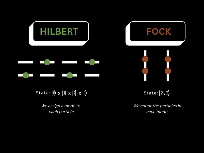
In this diagram, we can see the Hilbert and Fock space representation of the same state. The Hilbert space has a mode for each particle, but the Fock space counts the particles in each mode, it is in the state |2,2> which means we have two photons in the first mode and two in the second.
In the Hilbert space, each additional photon doubles our possible combinations, leading to a scaling of 2𝑛 where n is the number of photons. This follows from the fact that in our Hilbert space description of qubits, we take each qubit as a 2-level system, meaning each qubit adds 2 new degrees of freedom.
The limiting aspect of the Hilbert space qubit representation of quantum data is that it is only ever useful to model our qubits as a 2-level system, despite the number of available modes.
In the Fock space, our available combinations scale by a binomial factor of:
n is the number of photons and m is the number of modes.
It may not be immediately obvious why this is the case, so let’s examine the situation when we have 4 photons and 3 modes to distribute them between in Fock Space:
So in this case (n=4, m=3), We have 4 photons to be distributed among 3 modes. This problem now has the form of the famous stars and bars theorem.
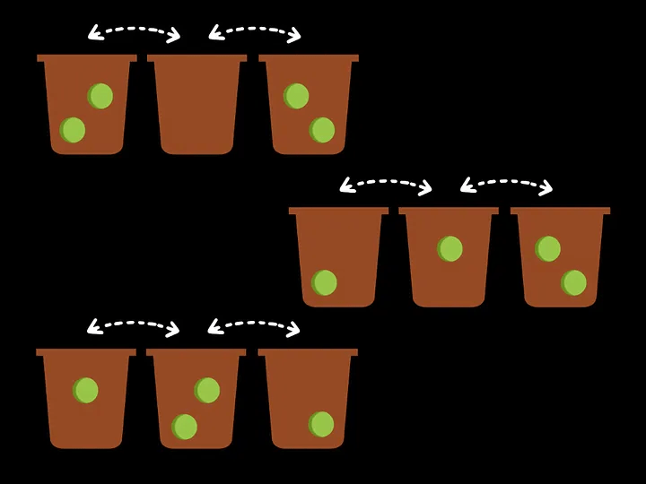
We can imagine that we have 4 indistinguishable balls that must be placed in 3 bins, and we must count all possible combinations. If we count the possibilities, we end up with
The stars and bars theorem states that this relationship always scales as a binomial coefficient. However, in experimental reality, it is not always possible to access every state in the Fock space. This is because we cannot always measure multiple photons in a single mode with perfect accuracy. This is an active area of research.
This scaling advantage for encoding our data into the photonic Fock space is shown for when the number of modes is twice the number of photons (m = 2n), in the following graph:

In summary, photonic devices allow us to access the Fock space which has a very useful scaling of the computational space. We should take advantage of this when designing algorithms to run on photonic quantum computers.
A Universal Function Approximator (Fourier Series)
A tremendously useful application of a photonic quantum circuit arranged in this way is that it can be used to simulate Fourier Series.
A Fourier series is an expansion of a mathematical function in terms of an infinite sum of sine and cosine functions.
To the non-mathematicians in the audience, this may not sound like a particularly exciting application, but those who have sweated through a multivariable analysis module know that these Fourier Series can be used to approximate ANY function defined over a given interval to an arbitrary degree of accuracy.
This means; if we can show that any Fourier Series can be generated by a quantum circuit then we have made a universal function generator.
A Fourier Series takes the form:
where x are our data points, cω are variable coefficients and ω are integer-valued multiples of a base frequency ω0. Ω is our range of frequencies.
In this paper, they discuss in detail the conditions necessary for a quantum circuit to universally express a Fourier series.
To briefly summarise: the more photons we send in, the more expressive the data encoding operation becomes, and the larger the available spectrum of the output function becomes.
Circuit description
Our quantum circuits look a bit like a classical Neural Network. In a traditional neural network, you have nodes or neurons connected by weights where you try to optimise these weights in order to minimise a cost function.
In ML, cost functions are used to estimate how badly models are performing. Put simply, a cost function is a measure of how wrong the model is in terms of its ability to estimate the relationship between the input of a function and its output. So the lower the value of the cost function the better our model is.
In traditional Machine learning, we would input data points into trainable circuit blocks which have a tunable parameter which we can adjust through multiple runs of our circuit to minimise our defined cost function.
So far, so classical.
What’s unique about our QML circuits is that our data is fed into a quantum circuit which encodes our data in to a quantum state (such as our Fock state) which is then manipulated by adjustable quantum gates. The parameters θ for these quantum gates are optimised using a classical algorithm and fed back into the quantum circuit to give us our ideal quantum output. This is illustrated in the diagram below:
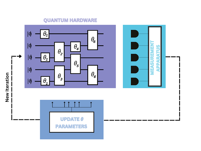
We can see that the parameters of our quantum gates are altered to give us our desired output. We refer to this as a hybrid algorithm as it makes use of both classical and quantum methods.
Classifier Algorithm
Everything we have discussed so far can be neatly implemented in to a QML — classifier algorithm.
A classifier algorithm is used to train a circuit to recognize and distinguish different categories of data. We will take a look at a two-dimensional binary classifier algorithm, which is the simplest example as it only distinguishes between two categories of data.
For the binary classifier algorithm, the objective is simple. We have a set of data, with elements belonging to one of two classes, Class A or Class B. We must train an algorithm to distinguish the difference.
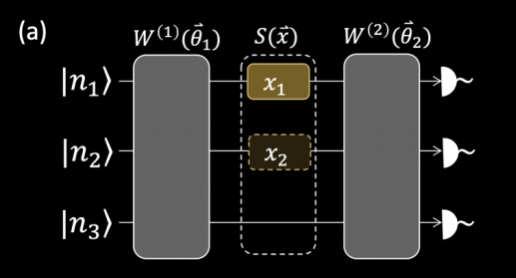
Our algorithm is based on the following circuit:
Data input and output
Like a typical ML algorithm, we first input training data. This is encoded by the S(x) blocks in to our Fock states:
where n is the number of photons sent into mode i. This data is manipulated by our training blocks W(θ) and outputs in the form of a Fourier Series f(xi), as discussed earlier.
Cost function
We then need to define and minimize a cost function to train our circuit with this training data. Our aim is that when we give the trained circuit some new test data, it will be able to categorize and divide it.
The test data has a predefined classification Yxi which defines the class it belongs to. So, our cost function then takes the form:
This is the difference between the values f (the classification to be predicted by our circuit) and y (the actual classification of the data). By tuning the parameters θ of the W(θ) blocks, our circuit can be trained to perfectly identify the training data by minimising this cost function as much as possible
By adapting the circuit to bring this cost function to a minimum, we have prepared a circuit that can output the correct classification of a given input.
Our circuit is then ready to classify some new test data. In the picture below, we can see an illustration of how the data may be classified and separated.
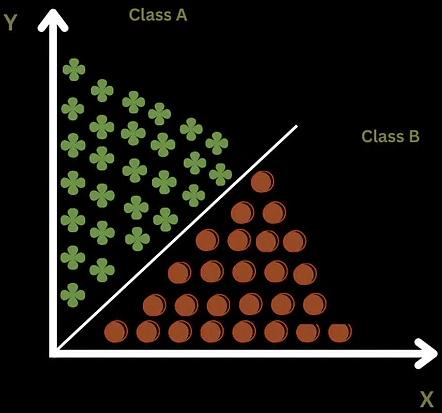
This is the simplest version of this type of algorithm, but it gives you an idea of what is possible. These algorithms are already being applied to applications such as the classification of different molecules. This could be very powerful for the discovery of new chemical products such as medicines.
QML Skepticism
For the sake of balance, it is worth noting that alongside the great enthusiasm for QML- techniques, there is some (valid) scepticism about the current hype surrounding the topic.
Maria Schuld and Nathan Killoran outline a number of criticisms of our current attitudes towards this field. They remind researchers to avoid the ‘tunnel vision of quantum advantage’.
It’s an astute point that many people are rushing to implement quantum versions of classical algorithms even if the quantum version might not be particularly useful. They can then try to get a better performance with the quantum algorithm and claim quantum advantage. Sometimes this increase in performance is obtained only on a specific dataset that is carefully chosen, or the classical counterpart could perform better if it was optimised more.
In the same way that quantum computers are not expected to be better than classical computers for all problems, but only for some specific ones (such as factoring with Shor’s algorithm), we expect that QML is going to beat ML only in specific scenarios. It is now up to the researchers to find the scenarios where QML will truly excel.

